simulate simple experiments, evaluate the simulated data with Python and visualise it with the help of coordinate graphics.
EXAMPLES
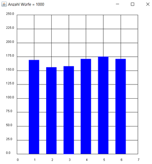
Example 1: Dice simulation
Using random numbers, you simulate the throwing of a dice. The randint(1, 6) function from the random module returns random dice numbers (1, 2, ...6). In your programme, 1000 such dice numbers are generated and the frequencies with which the individual numbers occur are recorded in a list p and displayed in a frequency diagram. p = [0] * 7 generates a list with 7 zeros.
Experiment with different n. The larger n, the more even the frequency distribution should be..
Program:
#Gp14.pyfrom gpanel import *
from random import randint
n = 1000
print("Anzahl Wuerfe = " + str(n))
makeGPanel(-1, 8, -2*n/100, n/4 + n/100)
drawGrid(0, 7, 0, n/4, 7, 10)p = [0] * 7repeat n:
a = randint(1, 6)if a == 1:
p[1] += 1
elif a == 2:
p[2] += 1
elif a == 3:
p[3] += 1
elif a == 4:
p[4] += 1
elif a == 5:
p[5] += 1
elif a == 6:
p[6] += 1
setColor("blue")
for i in range(1, 7):
fillRectangle(i-0.3 , 0, i + 0.3, p[i])
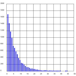
You throw a dice and ask yourself how many times you have to roll the dice on average until a certain number, e.g. a 6, appears. If you imagine that each roll takes the same amount of time, this is the average waiting time.
Instead of proceeding mathematically, simulate rolling the dice with random numbers 1, 2, 3, ... 6 and repeat this experiment until the number 6 occurs. The number of trials required is stored in the variable k. You repeat the experiment 10000 times and display the frequencies in a frequency diagram. At the same time, form the sum of k so that you can calculate the average waiting time at the end. This is shown in the title. To understand the simulation, first experiment with small n values (e.g. n = 5, n = 10, n = 100).
Program:
# Gp14a.pyfrom gpanel import *
from random import randint
n = 10000
def sim():
k = 1
r = randint(1, 6)
while r != 6:
r = randint(1, 6)
k += 1
return k
makeGPanel(-5, 55, -200, 2200)
drawGrid(0, 50, 0, 2000)
print("Waiting on a 6")
setColor("blue")
h = [0] * 51
lineWidth(5)
count = 0
repeat n:
k = sim()
print k
count += k
if k <= 50:
h[k] += 1
line(k, 0, k, h[k])
mean = count / n
print("Mean waiting time = " + str(mean))
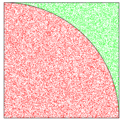
Example 3: Calculating the number PI using the Monte Carlo method
This is a classic example of a computer simulation. A large number n of random points are thrown onto a square with side length 1. The proportion of points within the quarter circle obviously corresponds approximately to its area.
If n points are thrown and the number of hits is inside the quarter circle, the following applies
hits / n = quarter circle area / square area
You can solve the problem graphically and mathematically using a GPanel. To generate the random points, use the random() function, which returns random numbers between 0 and 1 (with 12 decimal places).
Program:
# Gp14b.pyfrom gpanel import *
from random import random
makeGPanel(-0.3, 1.3, -0.3, 1.3)
rectangle(0, 0, 1, 1)
arc(1, 0, 90)
hits = 0
n = input("Number of rain drops")
i = 0
while i < n:
x = random()
y = random()
if x*x + y*y < 1:
hits = hits + 1
setColor("red")
else:
setColor("green")
i = i + 1
point(x, y)
pi = 4 * hits / nprint("Result: pi = " + str(pi))
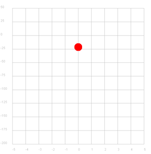
Example 4: Simulation of a vertical throw
With the acceleration a in a small time interval dt, the new velocity vneu = v + a * dt and the new location xneu = x + v * dt. Here the acceleration a = -g. The new state is calculated every 0.05 seconds.
Program:
# Gp14c.pyfrom gpanel import *
import time
makeGPanel(-130, 130, -170, 70)
setColor("red")
enableRepaint(False)
g = 9.81
dt= 0.05
t = 0; y = 0
v = 25
while t < 10:
v = v - g * dt
y = y + v * dt
t = t + dt
drawGrid(-100, 100, -150, 50, "gray")
pos(0, y)
fillCircle(5)
repaint()
time.sleep(dt)
clear()
You use random numbers for the simulation. The random() function from the random module returns random numbers with 12 decimal places that are greater than 0 and less than 1. The randint(a, b) function returns integer random numbers between a and b (limits included).
TO SOLVE BY YOURSELF
1)
In a game, 3 dice are thrown at the same time. Player A wins if at least one six is rolled. Player B wins if there is no six. Who has the better chance of winning if the game is repeated as often as desired?
2)
Ask yourself how often you have to roll the dice on average to get all the dice numbers 1, 2, 3, 4, 5, 6 at least once.
Solve the question with a simulation.
3)
Simulate the tossing of two coins and show the frequencies with which the events ‘twice tails’, ‘once tails and once heads’ and ‘twice heads’ occur in a frequency diagram.
4)
In example 4, a vertical wall is simulated. Similarly, you can also simulate an oblique throw. A body is thrown at an angle of 45° with an initial velocity of 32. Graph its trajectory for 10 seconds. To use the functions sin and cos, you must add the following import line: from math import sin, cos, pi
You can use example 4 as a template and replace the physical formula with those for the inclined throw:
g = 9.81
dt = 0.05
v = 32
alpha = pi/4

t = 0; x = 0; y = 0
vx = v * math.cos(alpha)
vy = v * math.sin(alpha)

while t < 10:
    vy = vy - g * dt
    x = x + vx * dt
    y = y + vy * dt
Note: The angle in the functions sin() and cos() must be specified in radians. pi/4 corresponds to the angle 45°. The radians(alpha) function, which converts angles in degrees to angles in radians, can be used for the conversion. This must also be imported.